Remasking Discrete Diffusion Models with Inference-Time Scaling

Masked discrete diffusion models have recently challenged the long-dominant next-token prediction autoregressive (AR) models in language modeling. Although masked diffusion models still slightly lag behind AR models regarding the quality of language distribution estimation, i.e., test perplexity, they hold several key advantages over AR models. First, masked diffusion models can flexibly change the number of model forward passes during sampling. One can either reduce the number of sampling steps for faster generation or increase this number to trade extra compute for better quality, i.e., conduct inference-time compute scaling. Second, when combined with diffusion guidance techniques, masked diffusion models are more adaptable to conditional generation.

However, one major drawback of previous masked diffusion models, which we refer to as the failure to remask property, has hindered the potentials mentioned above. To be more specific, in previous masked diffusion models, once a token is unmasked in the sampling process, it can never be masked or changed again. This property decides that no matter how many time steps are set for the sampling process, only the number of sequence length token predictions can be made, drastically restricting masked diffusion models' inference-time scaling capacity. Besides, this property also harms the model's controllability, since it cannot change the tokens generated at the early sampling phase even though they may have obstacled the desired holistic feature. In order to tackle this drawback, we propose ReMDM, a simple and general framework to design remasking samplers for masked diffusion models.

Given a clean one-hot representation of a data token \(\mathbf{x} \in \mathbb{R}^{|V|} \), where \(|V|\) denotes the vocabulary size, masked diffusion models design a forward Markov chain process \(q\) to gradually add noise to \(\mathbf{x}\) towards some limiting distribution \(\mathbf{m}\), which corresponds to a one-hot represesntation of a special \([MASK]\) token. Specifically, the forward process \(q\) is handcrafted and the marginal of each latent variable \(\mathbf{z}_t\) for \(t \in [0, 1]\), takes the following form. $$ q(\mathbf{z}_t|\mathbf{x}) = \mathrm{Cat}(\mathbf{z}_t;\alpha_t\mathbf{x} + (1 - \alpha_t)\mathbf{m}), $$ where \(\mathrm{Cat}\) denotes the categorical distribution and \(\alpha_t\) is a monotonically decreasing scalar variable with \(\alpha_0 \approx 1\) and \(\alpha_1 \approx 0\). Letting \(s\) denote the time step directly preceding \(t\), by Bayes' rule, the ground-truth posterior takes the following form: $$ q(\mathbf{z}_s|\mathbf{z}_t, \mathbf{x}) = \mathrm{Cat}(\mathbf{z}_s; \frac{\alpha_s - \alpha_t}{1 - \alpha_t}\mathbf{x} + \frac{1 - \alpha_s}{1 - \alpha_t}\mathbf{z}_t) $$ The goal of diffusion modeling is to learn a parameterized model \(p_\theta\) to fit the corresponding reverse process. We parameterize this model with a neural network \(\mathbf{x}_\theta(\mathbf{z}_t)\) that aims to recover \(\mathbf{x}\) given some noised latent at timestep \(t\), and we set the parameterized posterior as \(p_\theta(\mathbf{z}_s|\mathbf{z}_t) = q(\mathbf{z}_s|\mathbf{z}_t, \mathbf{x}_\theta(\mathbf{z}_t))\). To train the model, we use the technique of variational inference as in continuous diffusion models and minimize the following objective: $$ \mathcal{L} = \mathbb{E}_{t \in \{\frac{1}{T}, \ldots, 1\}, \mathbf{z}_{0:T} \sim q(\mathbf{z}_{0:T}|\mathbf{x})} \bigg[\underbrace{-\log p_\theta(\mathbf{x}|\mathbf{z}_0)}_{\mathcal{L}_{reconstruct}} + \underbrace{T\frac{\alpha_t - \alpha_s}{1-\alpha_t}\log(\mathbf{x}_\theta(\mathbf{z}_t)^\top\mathbf{x}))}_{\mathcal{L}_{diffusion}} + \underbrace{D_{KL}(q(\mathbf{z}_T|\mathbf{x})\Vert p_\theta(\mathbf{z}_T))}_{\mathcal{L}_{prior}}\bigg], $$ where \(T\) is the predefined number of sampling steps and \(D_{KL}\) denotes the compuation of KL divergence. Of note, the probability distribution at time \(T\) is a delta distribution centered at the \([MASK]\) token, rendering \(\mathcal{L}_{prior}\) as 0 and thus could be omitted. Following Sahoo et al. 2024, we refer to this model as MDLM.

Failure to remask property: Following the form for the posterior above, when \(\mathbf{z}_t \neq \mathbf{m}\), the distribution is a discrete delta function concentrated on \(\mathbf{z}_t=\mathbf{x}\). We thus have \(p_\theta(\mathbf{z}_s|\mathbf{z}_t) = \mathrm{Cat}(\mathbf{z}_s; \mathbf{z}_t)\), which implies that in the sampling process, once a token is unmasked, it stays unchanged until the end of the generation process. We refer to this as the failure to remask property.

In order to allow remasking sampling, we need to change the ground-truth posterior such that \(q(\mathbf{z}_s=\mathbf{m}|\mathbf{z}_t=\mathbf{x}, \mathbf{x}) > 0\). Apart from this, we want the whole system to be stable so that the least amount of modification is introduced. Observing the training objective function, we notice that it only depends on the forward marginal \(q(\mathbf{z}_t|\mathbf{x})\). Therefore, we would like the marginal to be unchanged when we modify the posterior. Given the two conditions discussed, we derive the new posterior as: $$ q_\sigma(\mathbf{z}_s|\mathbf{z}_t, \mathbf{x}) = \begin{cases} \mathrm{Cat}(\mathbf{z}_s; (1-\sigma_t)\mathbf{x} + \sigma_t\mathbf{m}), \quad \mathbf{z}_t \neq \mathbf{m} \\ \mathrm{Cat}(\mathbf{z}_s; \frac{\alpha_s - (1-\sigma_t)\alpha_t}{1-\alpha_t}\mathbf{x} + \frac{1-\alpha_s-\alpha_t\sigma_t}{1-\alpha_t}\mathbf{m}), \quad \mathbf{z}_t = \mathbf{m} \end{cases} $$ \(\sigma_t\) is a scalar parameter that we can control. Intuitively, it represents the probability of remasking an already generated token. In order to make the probability distribution mathematically valid, the four coefficients should all have the value between 0 and 1. This gives us the following constraint: $$ 0 \leq \sigma_t \leq min\{1, \frac{1 - \alpha_s}{\alpha_t}\} := \sigma_t^{max} $$ Note that this is the only constraint on \(\sigma_t\). This means that for a token at any position in the sequence and at any time step, we can choose its value as we want as long as it falls within the aforementioned interval. This gives us much flexibility in terms of sampler design. Considering the remasking property, we dub our method ReMasking Diffusion Models (ReMDM).

Now let's wrap up and summerize how to design a remasking sampler. Suppose that we already have a well-trained neural network \(\mathbf{x}_\theta\), we can first design a suitable remasking schecule \(\sigma_t\) and then plug \(\mathbf{x}_\theta\) into \(q(\mathbf{z}_s|\mathbf{z}_t, \mathbf{x})\) to get our parameterized posterior as \(p_\theta(\mathbf{z}_t|\mathbf{z}_s) = q(\mathbf{z}_s|\mathbf{z}_t, \mathbf{x}_\theta(\mathbf{z}_t))\). After this, we can begin the sampling process by starting with a token sequence filled with \([MASK]\) and then iteratively applying \(p_\theta(\mathbf{z}_s|\mathbf{z}_t)\) to it for \(T\) times to get our generated sample.

However, how to get the well-trained \(\mathbf{x}_\theta\) remains unsolved. Ideally, we should only train the model once and reuse the same neural network for samplers with different \(\sigma_t\) schedules. Here, we argue that we can reuse the MDLM checkpoint. To understand why we make this claim, let's revisit the training objective. After we change the original \(q\) into the remasking \(q_\sigma\), \(\mathcal{L}_{prior}\) and \(\mathcal{L}_{reconstruct}\) should stay the same since the marginal is unchanged. By applying \(q_\sigma\) and the corresponding \(p_\theta\), the diffusion loss becomes $$ \mathcal{L}_{diffusion}^\sigma = \mathbb{E}_{t \in \{\frac{1}{T}, \ldots, 1\}, \mathbf{z}_t \sim q(\mathbf{z}_t|\mathbf{x})}\bigg[T\frac{(1-\sigma_t)\alpha_t - \alpha_s}{1 - \alpha_t} \log(\mathbf{x}_\theta(\mathbf{z}_t)^\top \mathbf{x}) \bigg] $$ We first note that \(\mathcal{L}_{diffusion}^\sigma\) is a reweighted version of \(\mathcal{L}_{diffusion}\). Second, we observe that \(\mathcal{L}_{diffusion}^\sigma\) increases monotonically in \(\sigma_t\). Finally, when \(\sigma_t\) reaches it lower bound, i.e., 0, \(\mathcal{L}_{diffusion}^\sigma = \mathcal{L}_{diffusion}\). Combining these observations, we make the following claims: (1) ReMDM represents a family of discrete diffusion models with MDLM as its special case. (2) MDLM is the one that yields the tightest evidence lower bound. (3) Therefore, one can presumably reuse weights from an MDLM model, i.e., using different \(\sigma_t\) at training and inference. Indeed, we find this to be a performant strategy in practice.

ReMDM opens up a broad design space of remasking samplers with few constraints. Here, we explore some of them. We empirically find that for different tasks, different \(\sigma_t\) schedules work the best.

Max-capped Schedule. We can potentially reduce the maximum probability of remasking to a constant \(\eta_{cap} \in [0, 1]\). Concretely, we let \(\sigma_t = min\{\eta_{cap}, \frac{1-\alpha_s}{\alpha_t}\}\), for all \(t \in [0, 1]\). We denote this schedule as “ReMDM-cap.”

Rescaled Schedule. Alternatively, we can temper the chances of remasking by setting \(\sigma_t = \eta_{rescale}\cdot\sigma_{t}^{max}\), with \(\eta_{rescale} \in [0, 1]\) as a hyperparameter that controls this rescaling. We denote this schedule as “ReMDM-rescale.”

Confidence-Based Schedule. In conjunction with the two strategies above, we explore a further reweighing of \(\sigma_t\) which is based on the intuition that tokens of which the denoising model is less confident should be assigned a larger probability of remasking. In the previous part of this blog post, if \(t\) is fixed, then the \(\sigma_t\) value for each token in the sequence is the same. Now let's consider different \(\sigma_t\) for tokens at different positions. Consider the \(\ell\)-th token in a sequence of \(L\) latents at time \(t\). For each \(\ell \in \{1, \ldots, L\}\), we store its decoding probability at the time \(\tau\) at which it was last unmasked. Concretely, if \(\mathbf{z}_t^{(\ell)} \neq \mathbf{m}\), then we define \( \psi_t^{(\ell)} := \mathbf{x}_{\theta, \tau}^{(\ell)\top}\mathbf{z}_\tau^{(\ell)} \) If \(\mathbf{z}_t^{(\ell)} = \mathbf{m}\), then \( \psi_t^{(l)} := \infty\). Thus, \(\psi_t^{(\ell)}\) serves as a 'confidence score' for unmasked tokens. We then compute \(\sigma_t^{(\ell)} = \eta_{conf}^{\ell} \cdot \sigma_t\), where \(\eta_{conf}^{(\ell)} = \frac{\exp(-\psi_t^{(\ell)})}{\sum_{\ell^\prime=1}^L \exp(-\psi_{t}^{(\ell^\prime)})} \). With this schedule, masked tokens are decoded using the approximate posterior from MDLM, and the unmasked tokens are remasked negatively proportional to their confidence. We denote this schedule as “ReMDM-conf.”

So far, we have been applying remasking for all \(t \in [0, 1]\). However, there may be certain periods in the generation process when remasking is not necessary. For example, in the early phase of sampling when few tokens are unmasked, remasking them may do little good but slow down the generation. Therefore, we propose two methods for optionally 'turning on/off' ReMDM sampling, which amount to the following modification of the \(\sigma_t\) schedules above: $$ \tilde{\sigma}_t = \begin{cases} \sigma_t, & \text{if } t \in [t_{on}, t_{off}), \text{with } t_{on} > t_{off} \\ 0, & \text{otherwise}. \end{cases} $$ Switch. We choose some \(t_{switch} \in (0, 1]\) and we have \( [t_{on}, t_{off}) = [t_{switch}, 0) \). We denote this strategy as “ReMDM-switch.”

Loop. In this strategy, we set both \(t_{on}, t_{off} \in (0, 1] \). Furthermore, in the range when ReMDM is activated, we modify the noise schedule to be constant, such that \(\alpha_t = \alpha(t_{on})\). As shown in the figure below, this divides the sampling process into three phases. In the first phase, the model generates tokens without remasking (\(\sigma_t = 0\), i.e., using MDLM). In the second phase, we hold \(\alpha\) constant (i.e., \(\alpha_s = \alpha_t\)), and the model is asked to remask and predict a proportion of the generated tokens in a loop. In particular, one can use any ReMDM strategy introduced above in this phase. Intuitively, if a 'bad' token is remasked, it will likely be replaced with a 'good' token due to the abundant context. Even if a 'good' token happens to be remasked, since the signal-to-noise ratio is designed to be high in this portion of the generation process, it will likely be re-decoded as other (if not the same) 'good' tokens. In this way, ReMDM-loop corrects the 'bad' tokens and maintains the 'good' tokens, i.e., fixes mistakes. Finally, in the third phase, we let the model predict any remaining unmasked tokens using the MDLM posterior. We denote this strategy as “ReMDM -loop.”

Depiction of ReMDM-loop \(\alpha_t\) and \(\sigma_t\) schedules.

Previous works, e.g., the forward-backward (FB; Campbell et al. (2022)) and discrete flow matching (DFM; Gat et al., 2024) correctors, propose to tackle the failure to remask property with discrete predictor-corrector samplers, a special type of discrete diffusion samplers that decompose a single sampling step into one predictor step followed by a certain number of corrector steps that remediate possible mistakes without changing the marginals. Here, we demonstrate that these methods are special cases of ReMDM

Proposition 1. The FB corrector on MDLM is a special case of ReMDM where \(\sigma_t = \frac{\alpha_s - \alpha_t}{\alpha_t}\).
Proposition 2. The DFM corrector on MDLM is a special case of ReMDM where \(\alpha_t = \frac{\beta_t(\alpha_s - \alpha_t)}{\alpha_t}\). \(\beta_t \in \mathbb{R}\) denotes the corrector schecule.
Proposition 2 ensures that any DFM corrector can be transformed into a ReMDM sampler, which shows that DFM corrector is a subset of ReMDM. The following proposition proves that this subset is proper.
Proposition 3. The ReMDM sampler is more general than DFM corrector, since only the former can accommodate noise schedules with constant \(\alpha_t\) for some range \([t, t - \Delta t]\) where \(\Delta t > 0\).

Unconditional text generation on OpenWebText

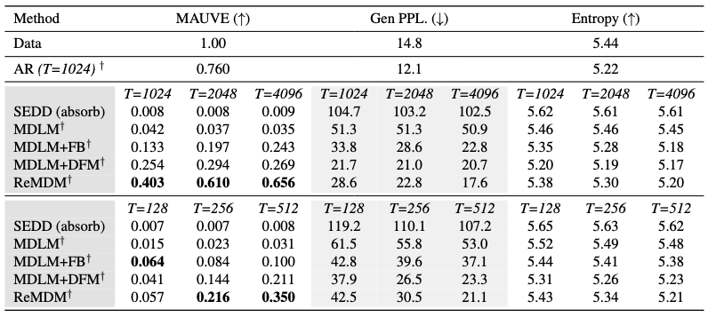
We test ReMDM's text generation capacity with unconditoinal generation from models trained on OpenWebText. We report the MAUVE score as the main metric due to the generative perplexity (Gen PPL.) hacking phenomenon (see Section 5.1.1 in the paper for more details). Note that Gen PPL. and entropy are only reported for completeness and that lower Gen PPL. does not always correlate with better quality. We examine two settings: (1) inference-time scaling (\(T \geq L=1024\)) and (2) faster sampling (\(T < L=1024\)). In both settings, ReMDM achieves the best performance. Notably, ReMDM scales favorably with inference-time compute. In contrast, masked diffusion models scale poorly with \(T\), and corrector sampler methods saturate when \(T\) is large.

ReMDM improves sample quality in the case of inference-time scaling and faster sampling. ReMDM outperforms state-of-the-art masked diffusion models (SEDD; Lou et al. (2024), MDLM; Sahoo et al. (2024)) and masked diffusion models with corrector samplers such as Forward-Backward (FB; Campbell et al. (2022)) and Discrete Flow Matching (DFM; Gat et al. (2024)) corrector samplers. \(^{\dagger}\) indicates nucleus sampling (top-p=0.9). For each \(T\), the best diffusion MAUVE score is bolded.

Class-conditioned image generation on ImageNet 256\(\times\)256

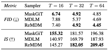
We use a pretrained MaskGiT model (Chang et al., 2022) that was trained on ImageNet samples with 256\(\times\)256 pixels. For each experiment, we use a different sampler (MaskGiT, MDLM, or ReMDM) and generate 50,000 images conditioned on randomly sampled class labels. We measure sample quality using Fréchet Inception Distance (FID) and Inception Score (IS) and report the best setting for each method. Although for the smallest \(T\) decoding setting MaskGiT outperforms the other methods, we see that ReMDM has the best scaling, producing the highest quality images of any model at \(T = 64\).

ReMDM produces the highest quality images. Values reflect FID / IS for varying \(T\) on discretized ImageNet conditional generation. For each metric and \(T\), the best value is bolded.

Conditional QM9 molecule generation

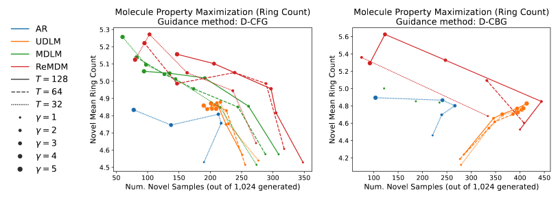
We follow the setup from Schiff et al. (2024) to explore controlled small molecule generation. We use the discrete classifier-free guidance (D-CFG) and discrete classifier-based guidance (D-CBG) methods defined in Schiff et al. (2024) to conditionally generate molecules with higher ring counts (greater than 90th percentile in the original dataset) on top of AR, MDLM, ReMDM and UDLM (state-of-the-art uniform noise discrete diffusion models proposed in Schiff et al. (2024)). For D-CBG on AR, we use the popular FUDGE (Yang & Klein, 2021) method. In the following figure, we display the trade-off that comes from increasing guidance strength \(\gamma\). We only visualize results for samples that had at least 50 novel sequences. For both forms of guidance, D-CFG and D-CBG, ReMDM outperforms AR and diffusion approaches, pushing the novelty-property maximization frontier beyond that of the baseline methods. Additionally, ReMDM scales favorably with more inference-time compute, seen by the curves for larger T dominating those for smaller T.

ReMDM improves steerability by extending the novelty-property maximization frontier. Controlled generation for ring count maximization on QM9 dataset with varying inference compute \(T\) and guidance strength \(\gamma\). (Left) Discrete classifier-free guidance (D-CFG). (Right) Discrete classifier-based guidance (D-CBG) and FUDGE for AR.

Downstream task performance

Recent diffusion large language models (dLLMs) such as LLaDA 8B Nie et al. (2024) and Dream 7B Nie et al. (2024) have demonstrated on par downstream task performance with autoregressive language models of the same parameter scale. However, these dLLMs still suffer from the failure to remask property. Therefore, we test the effect of remasking sampling on dLLLMs on Countdown (bidirectional reasoning) and TruthfulQA (factual knowledge grasp). In both of the settings, we use few-shot evaluation (4-shot for Countdown, and 6-shot for TruthfulQA). In Countdown, pass@1 is reported and in TruthfulQA, the ROUGE score differences between the model and correct answers and model and plausibly wrong answers provided by the dataset are reported. For both of the metrics, we report their mean values and 95% confidence intervals of 20 experiment runs with different random seeds. As shown in the following table, LLaDA with ReMDM consistently performs the best and exceeds the original LLaDA with statistical significance.

LLaDA with ReMDM performs the best on downstream tasks, and consistently exceeds the original LLaDA with statistical significance. For each metric, the best value is bolded.

In this work, we have presented a novel family of absorbing state discrete diffusion samplers. Our method leverages the strong language modeling performance of this class of models by enabling the use of pretrained weights with the added benefit of more flexible sampling strategies that allow for remasking of predicted tokens. We demonstrate empirically that this leads to improved sample quality for both unconditional and conditional generation. Our approach also unlocks an important inference-time compute scaling axis that is more limited for existing masked diffusion models.